Readme:
Appendix:
LexicalRichness Documentation
Useful Links
LexicalRichness


LexicalRichness is a small Python module to compute textual lexical richness (aka lexical diversity) measures.
Lexical richness refers to the range and variety of vocabulary deployed in a text by a speaker/writer (McCarthy and Jarvis 2007) . Lexical richness is used interchangeably with lexical diversity, lexical variation, lexical density, and vocabulary richness and is measured by a wide variety of indices. Uses include (but not limited to) measuring writing quality, vocabulary knowledge (Šišková 2012) , speaker competence, and socioeconomic status (McCarthy and Jarvis 2007). See the notebook for examples.
1. Installation
Install using PIP
pip install lexicalrichness
If you encounter,
ModuleNotFoundError: No module named 'textblob'
install textblob:
pip install textblob
Note: This error should only exist for versions <= v0.1.3. Fixed in
v0.1.4 by David Lesieur and Christophe Bedetti.
Install from Conda-Forge
LexicalRichness is now also available on conda-forge. If you have are using the Anaconda or Miniconda distribution, you can create a conda environment and install the package from conda.
conda create -n lex
conda activate lex
conda install -c conda-forge lexicalrichness
Note: If you get the error CommandNotFoundError: Your shell has not been properly configured to use 'conda activate' with conda activate lex in Bash either try
conda activate bashin the Anaconda Prompt and then retryconda activate lexin Bashor just try
source activate lexin Bash
Install manually using Git and GitHub
git clone https://github.com/LSYS/LexicalRichness.git
cd LexicalRichness
pip install .
Run from the cloud
Try the package on the cloud (without setting anything up on your local machine) by clicking the icon here:
![]()
2. Quickstart
>>> from lexicalrichness import LexicalRichness

# text example
>>> text = """Measure of textual lexical diversity, computed as the mean length of sequential words in
                a text that maintains a minimum threshold TTR score.

                Iterates over words until TTR scores falls below a threshold, then increase factor
                counter by 1 and start over. McCarthy and Jarvis (2010, pg. 385) recommends a factor
                threshold in the range of [0.660, 0.750].
                (McCarthy 2005, McCarthy and Jarvis 2010)"""

# instantiate new text object (use the tokenizer=blobber argument to use the textblob tokenizer)
>>> lex = LexicalRichness(text)

# Return word count.
>>> lex.words
57

# Return (unique) word count.
>>> lex.terms
39

# Return type-token ratio (TTR) of text.
>>> lex.ttr
0.6842105263157895

# Return root type-token ratio (RTTR) of text.
>>> lex.rttr
5.165676192553671

# Return corrected type-token ratio (CTTR) of text.
>>> lex.cttr
3.6526846651686067

# Return mean segmental type-token ratio (MSTTR).
>>> lex.msttr(segment_window=25)
0.88

# Return moving average type-token ratio (MATTR).
>>> lex.mattr(window_size=25)
0.8351515151515151

# Return Measure of Textual Lexical Diversity (MTLD).
>>> lex.mtld(threshold=0.72)
46.79226361031519

# Return hypergeometric distribution diversity (HD-D) measure.
>>> lex.hdd(draws=42)
0.7468703323966486

# Return voc-D measure.
>>> lex.vocd(ntokens=50, within_sample=100, iterations=3)
46.27679899103406

# Return Herdan's lexical diversity measure.
>>> lex.Herdan
0.9061378160786574

# Return Summer's lexical diversity measure.
>>> lex.Summer
0.9294460323356605

# Return Dugast's lexical diversity measure.
>>> lex.Dugast
43.074336212149774

# Return Maas's lexical diversity measure.
>>> lex.Maas
0.023215679867353005

# Return Yule's K.
>>> lex.yulek
153.8935056940597

# Return Yule's I.
>>> lex.yulei
22.36764705882353

# Return Herdan's Vm.
>>> lex.herdanvm
0.08539428890448784

# Return Simpson's D.
>>> lex.simpsond
0.015664160401002505
3. Use LexicalRichness in your own pipeline
LexicalRichness comes packaged with minimal preprocessing + tokenization for a quick start.
But for intermediate users, you likely have your preferred nlp_pipeline:
# Your preferred preprocessing + tokenization pipeline
def nlp_pipeline(text):
    ...
    return list_of_tokens
Use LexicalRichness with your own nlp_pipeline:
# Initiate new LexicalRichness object with your preprocessing pipeline as input
lex = LexicalRichness(text, preprocessor=None, tokenizer=nlp_pipeline)

# Compute lexical richness
mtld = lex.mtld()
Or use LexicalRichness at the end of your pipeline and input the list_of_tokens with preprocessor=None and tokenizer=None:
# Preprocess the text
list_of_tokens = nlp_pipeline(text)

# Initiate new LexicalRichness object with your list of tokens as input
lex = LexicalRichness(list_of_tokens, preprocessor=None, tokenizer=None)

# Compute lexical richness
mtld = lex.mtld()
4. Using with Pandas
Here’s a minimal example using lexicalrichness with a Pandas dataframe with a column containing text:
def mtld(text):
    lex = LexicalRichness(text)
    return lex.mtld()

df['mtld'] = df['text'].apply(mtld)
5. Attributes
|
list of words |
|
number of words (w) |
|
number of unique terms (t) |
|
preprocessor used |
|
tokenizer used |
|
type-token ratio computed as t / w (Chotlos 1944, Templin 1957) |
|
root TTR computed as t / sqrt(w) (Guiraud 1954, 1960) |
|
corrected TTR computed as t / sqrt(2w) (Carrol 1964) |
|
log(t) / log(w) (Herdan 1960, 1964) |
|
log(log(t)) / log(log(w)) (Summer 1966) |
|
(log(w) ** 2) / (log(w) - log(t) (Dugast 1978) |
|
(log(w) - log(t)) / (log(w) ** 2) (Maas 1972) |
|
Yule’s K (Yule 1944, Tweedie and Baayen 1998) |
|
Yule’s I (Yule 1944, Tweedie and Baayen 1998) |
|
Herdan’s Vm (Herdan 1955, Tweedie and Baayen 1998) |
|
Simpson’s D (Simpson 1949, Tweedie and Baayen 1998) |
6. Methods
|
Mean segmental TTR (Johnson 1944) |
|
Moving average TTR (Covington 2007, Covington and McFall 2010) |
|
Measure of Lexical Diversity (McCarthy 2005, McCarthy and Jarvis 2010) |
|
HD-D (McCarthy and Jarvis 2007) |
|
voc-D (Mckee, Malvern, and Richards 2010) |
|
Utility to plot empirical voc-D curve |
Plot the empirical voc-D curve
lex.vocd_fig(
    ntokens=50,  # Maximum number for the token/word size in the random samplings
    within_sample=100,  # Number of samples
    seed=42,  # Seed for reproducibility
)
Assessing method docstrings
>>> import inspect

# docstring for hdd (HD-D)
>>> print(inspect.getdoc(LexicalRichness.hdd))

Hypergeometric distribution diversity (HD-D) score.

For each term (t) in the text, compute the probabiltiy (p) of getting at least one appearance
of t with a random draw of size n < N (text size). The contribution of t to the final HD-D
score is p * (1/n). The final HD-D score thus sums over p * (1/n) with p computed for
each term t. Described in McCarthy and Javis 2007, p.g. 465-466.
(McCarthy and Jarvis 2007)

Parameters
__________
draws: int
    Number of random draws in the hypergeometric distribution (default=42).

Returns
_______
float
Alternatively, just do
>>> print(lex.hdd.__doc__)

Hypergeometric distribution diversity (HD-D) score.

    For each term (t) in the text, compute the probabiltiy (p) of getting at least one appearance
    of t with a random draw of size n < N (text size). The contribution of t to the final HD-D
    score is p * (1/n). The final HD-D score thus sums over p * (1/n) with p computed for
    each term t. Described in McCarthy and Javis 2007, p.g. 465-466.
    (McCarthy and Jarvis 2007)

    Parameters
    ----------
    draws: int
        Number of random draws in the hypergeometric distribution (default=42).

    Returns
    -------
    float
7. Formulation & Algorithmic Details
For details under the hood, please see this section in the docs (or see here).
8. Example use cases
[1] SENTiVENT used the metrics that LexicalRichness provides to estimate the classification difficulty of annotated categories in their corpus (Jacobs & Hoste 2020). The metrics show which categories will be more difficult for modeling approaches that rely on linguistic inputs because greater lexical diversity means greater data scarcity and more need for generalization. (h/t Gilles Jacobs)
Jacobs, Gilles, and Véronique Hoste. “SENTiVENT: enabling supervised information extraction of company-specific events in economic and financial news.” Language Resources and Evaluation (2021): 1-33.
Click here for citation metadata
@article{jacobs2021sentivent,
        title={SENTiVENT: enabling supervised information extraction of company-specific events in economic and financial news},
        author={Jacobs, Gilles and Hoste, V{\'e}ronique},
        journal={Language Resources and Evaluation},
        pages={1--33},
        year={2021},
        publisher={Springer}
}
- [2] Shades of Neutrality: Detecting Media Slant in a Political Monopoly Using Quotation Accuracy. This paper develops quotation accuracy as a dimension of media slant. As covariates, I use characteristics of the text data (political speech and news article transcripts), one of which is lexical richness. Published in ACM Transactions on Intelligent Systems and Technology (2026).
Shen, Lucas (2026). Shades of Neutrality [Click for metadata]
@article{shen2026shades,
title={Shades of Neutrality: Detecting Media Slant in a Political Monopoly Using Quotation Accuracy},
author={Shen, Lucas},
journal={ACM Transactions on Intelligent Systems and Technology},
year={2026},
publisher={Association for Computing Machinery},
doi={10.1145/3787455},
url={https://doi.org/10.1145/3787455}
}
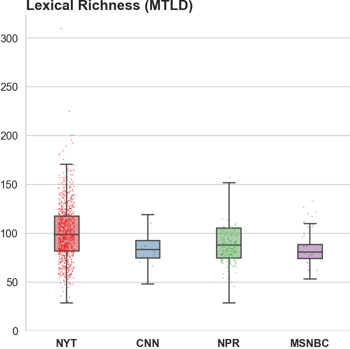
[3] Unreadable News: How Readable is American News? This study characterizes modern news by readability and lexical richness. Focusing on the NYT, they find increasing readability and lexical richness, suggesting that NYT feels competition from alternative sources to be accessible while maintaining its key demographic of college-educated Americans.
[4] German is more complicated than English This study analyses a small sample of English books and compares them to their German translation. Within the sample, it can be observed that the German translations tend to be shorter in length, but contain more unique terms than their English counterparts. LexicalRichness was used to generate the statistics modeled within the study.

9. Contributing
Author
Contributors
Contributions are welcome, and they are greatly appreciated! Every little bit helps, and credit will always be given. See here for how to contribute to this project. See here for Contributor Code of Conduct.
If you’d like to contribute via a Pull Request (PR), feel free to open an issue on the Issue Tracker to discuss the potential contribution via a PR.
10. Citing
If you have used this codebase and wish to cite it, here is the citation metadata.
Codebase:
@misc{lex,
        author = {Shen, Lucas},
        doi = {10.5281/zenodo.6607007},
        license = {MIT license},
        title = {{LexicalRichness: A small module to compute textual lexical richness}},
        url = {https://github.com/LSYS/lexicalrichness},
        year = {2022}
}
Documentation on formulations and algorithms:
@misc{accuracybias,
title={Measuring Political Media Slant Using Text Data},
author={Shen, Lucas},
url={https://www.lucasshen.com/research/media.pdf},
year={2021}
}
Published version of the above:
@article{shen2026shades,
title={Shades of Neutrality: Detecting Media Slant in a Political Monopoly Using Quotation Accuracy},
author={Shen, Lucas},
journal={ACM Transactions on Intelligent Systems and Technology},
year={2026},
publisher={Association for Computing Machinery},
doi={10.1145/3787455},
url={https://doi.org/10.1145/3787455}
}
The package is released under the MIT License.
Contributors
Author
Contributors
(See the Contributors page)
Details of Lexical Richness Measures
The two fundamental building blocks of all the measures are:
the total number of words in the text (w) , and
the number of unique terms (t).
TTR: Type-Token Ratio (Chotlos 1944, Templin 1957)

RTTR: Root Type-Token Ratio (Guiraud 1954, 1960)

CTTR: Corrected Type-Token Ratio (Carrol 1964)

Herdan: Herdan’s C (Herdan 1960, 1964)

Summer: Summer (Summer 1966)

Dugast: Dugast (Dugast 1978)

Maas: Maas (Maas 1972)

Yule’s K (Yule 1944, Tweedie and Baayen 1998)

Yule’s I (Yule 1944, Tweedie and Baayen 1998)

Herdan’s Vm (Herdan 1955, Tweedie and Baayen 1998)

Simpson’s D (Simpson 1949, Tweedie and Baayen 1998)

Attributes and Methods in LexicalRichness
This addendum exposes the underlying lexicalrichness measures from attributes and methods in the LexicalRichness class.
TTR: Type-Token Ratio (Chotlos 1944, Templin 1957)
- lexicalrichness.LexicalRichness.ttr()
Type-token ratio (TTR) computed as t/w, where t is the number of unique terms/vocab, and w is the total number of words. (Chotlos 1944, Templin 1957)
- Returns:
Type-token ratio
- Return type:
Float
RTTR: Root Type-Token Ratio (Guiraud 1954, 1960)]
- lexicalrichness.LexicalRichness.rttr()
Root TTR (RTTR) computed as t/sqrt(w), where t is the number of unique terms/vocab, and w is the total number of words. Also known as Guiraud’s R and Guiraud’s index. (Guiraud 1954, 1960)
- Returns:
Root type-token ratio
- Return type:
FLoat
CTTR: Corrected Type-Token Ratio (Carrol 1964)
- lexicalrichness.LexicalRichness.cttr()
Corrected TTR (CTTR) computed as t/sqrt(2 * w), where t is the number of unique terms/vocab, and w is the total number of words. (Carrol 1964)
- Returns:
Corrected type-token ratio
- Return type:
Float
Herdan: Herdan’s C (Herdan 1960, 1964)
- lexicalrichness.LexicalRichness.Herdan()
Computed as log(t)/log(w), where t is the number of unique terms/vocab, and w is the total number of words. Also known as Herdan’s C. (Herdan 1960, 1964)
- Returns:
Herdan’s C
- Return type:
Float
Summer: Summer (Summer 1966)
- lexicalrichness.LexicalRichness.Summer()
Computed as log(log(t)) / log(log(w)), where t is the number of unique terms/vocab, and w is the total number of words. (Summer 1966)
- Returns:
Summer
- Return type:
Float
Dugast: Dugast (Dugast 1978)
- lexicalrichness.LexicalRichness.Dugast()
Computed as (log(w) ** 2) / (log(w) - log(t)), where t is the number of unique terms/vocab, and w is the total number of words. (Dugast 1978)
- Returns:
Dugast
- Return type:
Float
Maas: Maas (Maas 1972)
- lexicalrichness.LexicalRichness.Maas()
Maas’s TTR, computed as (log(w) - log(t)) / (log(w) * log(w)), where t is the number of unique terms/vocab, and w is the total number of words. Unlike the other measures, lower maas measure indicates higher lexical richness. (Maas 1972)
- Returns:
Maas
- Return type:
Float
yulek: Yule’s K (Yule 1944, Tweedie and Baayen 1998)
- lexicalrichness.LexicalRichness.yulek()
Yule’s K (Yule 1944, Tweedie and Baayen 1998).
See also
frequency_wordfrequency_tableGet table of i frequency and number of terms that appear i times in text of length N.
- Returns:
Yule’s K
- Return type:
Float
yulei: Yule’s I (Yule 1944, Tweedie and Baayen 1998)
- lexicalrichness.LexicalRichness.yulei()
Yule’s I (Yule 1944).
See also
frequency_wordfrequency_tableGet table of i frequency and number of terms that appear i times in text of length N.
- Returns:
Yule’s I
- Return type:
Float
Herdan’s Vm (Herdan 1955, Tweedie and Baayen 1998)
- lexicalrichness.LexicalRichness.herdanvm()
Herdan’s Vm (Herdan 1955, Tweedie and Baayen 1998)
See also
frequency_wordfrequency_tableGet table of i frequency and number of terms that appear i times in text of length N.
- Returns:
Herdan’s Vm
- Return type:
Float
Simpson’s D (Simpson 1949, Tweedie and Baayen 1998)
- lexicalrichness.LexicalRichness.simpsond()
Simpson’s D (Simpson 1949, Tweedie and Baayen 1998)
See also
frequency_wordfrequency_tableGet table of i frequency and number of terms that appear i times in text of length N.
- Returns:
Simpson’s D
- Return type:
Float
msttr: Mean Segmental Type-Token Ratio (Johnson 1944)
- lexicalrichness.LexicalRichness.msttr(self, segment_window=100, discard=True)
Mean segmental TTR (MSTTR) computed as average of TTR scores for segments in a text.
Split a text into segments of length segment_window. For each segment, compute the TTR. MSTTR score is the sum of these scores divided by the number of segments. (Johnson 1944)
See also
segment_generatorSplit a list into s segments of size r (segment_size).
- Parameters:
segment_window (int) – Size of each segment (default=100).
discard (bool) – If True, discard the remaining segment (e.g. for a text size of 105 and a segment_window of 100, the last 5 tokens will be discarded). Default is True.
- Returns:
Mean segmental type-token ratio (MSTTR)
- Return type:
float
mattr: Moving Average Type-Token Ratio (Covington 2007, Covington and McFall 2010)
- lexicalrichness.LexicalRichness.mattr(self, window_size=100)
Moving average TTR (MATTR) computed using the average of TTRs over successive segments of a text.
Estimate TTR for tokens 1 to n, 2 to n+1, 3 to n+2, and so on until the end of the text (where n is window size), then take the average. (Covington 2007, Covington and McFall 2010)
See also
list_sliding_windowReturns a sliding window generator (of size window_size) over a sequence
- Parameters:
window_size (int) – Size of each sliding window.
- Returns:
Moving average type-token ratio (MATTR)
- Return type:
float
mtld: Measure of Textual Lexical Diversity (McCarthy 2005, McCarthy and Jarvis 2010)
- lexicalrichness.LexicalRichness.mtld(self, threshold=0.72)
Measure of textual lexical diversity, computed as the mean length of sequential words in a text that maintains a minimum threshold TTR score.
Iterates over words until TTR scores falls below a threshold, then increase factor counter by 1 and start over. McCarthy and Jarvis (2010, pg. 385) recommends a factor threshold in the range of [0.660, 0.750]. (McCarthy 2005, McCarthy and Jarvis 2010)
- Parameters:
threshold (float) – Factor threshold for MTLD. Algorithm skips to a new segment when TTR goes below the threshold (default=0.72).
- Returns:
Measure of textual lexical diversity (MTLD)
- Return type:
float
hdd: Hypergeometric Distribution Diversity (McCarthy and Jarvis 2007)
- lexicalrichness.LexicalRichness.hdd(self, draws=42)
Hypergeometric distribution diversity (HD-D) score.
For each term (t) in the text, compute the probabiltiy (p) of getting at least one appearance of t with a random draw of size n < N (text size). The contribution of t to the final HD-D score is p * (1/n). The final HD-D score thus sums over p * (1/n) with p computed for each term t. Described in McCarthy and Javis 2007, p.g. 465-466. (McCarthy and Jarvis 2007)
- Parameters:
draws (int) – Number of random draws in the hypergeometric distribution (default=42).
- Returns:
Hypergeometric distribution diversity (HD-D) score
- Return type:
float
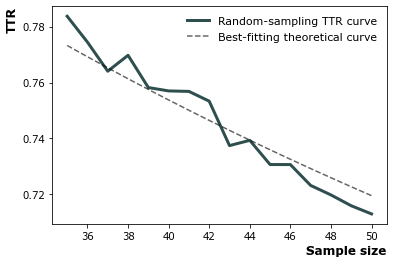
vocd: vod-D (Mckee, Malvern, and Richards 2010)
- lexicalrichness.LexicalRichness.vocd(self, ntokens=50, within_sample=100, iterations=3, seed=42)
Vocd score of lexical diversity derived from a series of TTR samplings and curve fittings.
Vocd is meant as a measure of lexical diversity robust to varying text lengths. See also hdd. The vocd is computed in 4 steps as follows.
Step 1: Take 100 random samples of 35 words from the text. Compute the mean TTR from the 100 samples.
Step 2: Repeat this procedure for samples of 36 words, 37 words, and so on, all the way to ntokens (recommended as 50 [default]). In each iteration, compute the TTR. Then get the mean TTR over the different number of tokens. So now we have an array of averaged TTR values for ntoken=35, ntoken=36,…, and so on until ntoken=50.
Step 3: Find the best-fitting curve from the empirical function of TTR to word size (ntokens). The value of D that provides the best fit is the vocd score.
Step 4: Repeat steps 1 to 3 for x number (default=3) of times before averaging D, which is the returned value.
See also
ttr_ndTTR as a function of latent lexical diversity (d) and text length (n).
- Parameters:
ntokens (int) – Maximum number for the token/word size in the random samplings (default=50).
within_sample (int) – Number of samples for each token/word size (default=100).
iterations (int) – Number of times to repeat steps 1 to 3 before averaging (default=3).
seed (int) – Seed for the pseudo-random number generator in ramdom.sample() (default=42).
- Returns:
voc-D
- Return type:
float
Helper: lexicalrichness.segment_generator
- lexicalrichness.segment_generator(List, segment_size)
Split a list into s segments of size r (segment_size).
- Parameters:
List (list) – List of items to be segmented.
segment_size (int) – Size of each segment.
- Yields:
List – List of s lists of with r items in each list.
Helper: lexicalrichness.list_sliding_window
- lexicalrichness.list_sliding_window(sequence, window_size=2)
Return a sliding window generator (of size window_size) over a sequence.
Taken from https://docs.python.org/release/2.3.5/lib/itertools-example.html.
Example:
List = [‘a’, ‘b’, ‘c’, ‘d’]
window_size = 2
- list_sliding_window(List, 2) ->
(‘a’, ‘b’)
(‘b’, ‘c’)
(‘c’, ‘d’)
- Parameters:
sequence (sequence (string, unicode, list, tuple, etc.)) – Sequence to be iterated over. window_size=1 is just a regular iterator.
window_size (int) – Size of each window.
- Yields:
List – List of tuples of start and end points.
Helper: lexicalrichness.frequency_wordfrequency_table
- lexicalrichness.frequency_wordfrequency_table(bow)
Get table of i frequency and number of terms that appear i times in text of length N.
For Yule’s I, Yule’s K, and Simpson’s D.
In the returned table, freq column indicates the number of frequency of appearance in the text. fv_i_N column indicates the number of terms in the text of length N that appears freq number of times.
- Parameters:
bow (array-like) – List of words
- Return type:
pandas.core.frame.DataFrame