Notebook Example
[1]:
from lexicalrichness import LexicalRichness
import lexicalrichness
lexicalrichness.__version__
[1]:
'0.4.0'
[2]:
# Enter your own text here if you prefer
text = """Measure of textual lexical diversity, computed as the mean length of sequential words in
                a text that maintains a minimum threshold TTR score.

                Iterates over words until TTR scores falls below a threshold, then increase factor
                counter by 1 and start over. McCarthy and Jarvis (2010, pg. 385) recommends a factor
                threshold in the range of [0.660, 0.750].
                (McCarthy 2005, McCarthy and Jarvis 2010)"""

# instantiate new text object (use the tokenizer=blobber argument to use the textblob tokenizer)
lex = LexicalRichness(text)
Attributes
[3]:
# Get list of words
list_of_words = lex.wordlist
print(list_of_words[:10], list_of_words[-10:])
['measure', 'of', 'textual', 'lexical', 'diversity', 'computed', 'as', 'the', 'mean', 'length'] ['factor', 'threshold', 'in', 'the', 'range', 'of', 'mccarthy', 'mccarthy', 'and', 'jarvis']
[4]:
# Return word count (w).
lex.words
[4]:
57
[5]:
# Return (unique) word count (t).
lex.terms
[5]:
39
Type-token ratio (TTR; Chotlos 1944, Templin 1957):
where \(t\) or \(t(w)\) is the number unique terms as function of the text of length \(w\) words.
[6]:
# Return type-token ratio (TTR) of text.
lex.ttr
[6]:
0.6842105263157895
Root TTR (RTTR; Guiraud 1954, 1960):
[7]:
# Return root type-token ratio (RTTR) of text.
lex.rttr
[7]:
5.165676192553671
Corrected TTR (RTTR; Guiraud 1954, 1960):
[8]:
# Return corrected type-token ratio (CTTR) of text.
lex.cttr
[8]:
3.6526846651686067
Herdan’s C (Herdan 1960, 1964):
[9]:
# Return Herdan's C
lex.Herdan
[9]:
0.9061378160786574
Summer’s index (Summer 1966)
[10]:
# Return Summer's index
lex.Summer
[10]:
0.9294460323356605
Dugast’s index (Dugast 1978):
[11]:
# Return Dugast's index
lex.Dugast
[11]:
43.074336212149774
Maas’s index (Maas 1972):
[12]:
lex.Maas
[12]:
0.023215679867353005
Yule’s K (Yule 1944, Tweedie and Baayen 1998):
[13]:
lex.yulek
[13]:
153.8935056940597
Yule’s I (Yule 1944, Tweedie and Baayen 1998):
[14]:
lex.yulei
[14]:
22.36764705882353
Herdan’s Vm (Herdan 1955, Tweedie and Baayen 1998):
[15]:
lex.herdanvm
[15]:
0.08539428890448784
Simpson’s D (Simpson 1949, Tweedie and Baayen 1998):
[16]:
lex.simpsond
[16]:
0.015664160401002505
Methods
MSTTR: Mean segmental type-token ratio
computed as average of TTR scores for segments in a text
Split a text into segments of length segment_window. For each segment, compute the TTR. MSTTR score is the sum of these scores divided by the number of segments
(Johnson 1944)
[17]:
lex.msttr(
    segment_window=25  # size of each segment
)
[17]:
0.88
MATTR: Moving average type-token ratio
Computed using the average of TTRs over successive segments of a text
Then take the average of all window’s TTR
(Covington 2007, Covington and McFall 2010)
[18]:
# Return moving average type-token ratio (MATTR).
lex.mattr(
    window_size=25  # Size of each sliding window
)
[18]:
0.8351515151515151
MTLD: Measure of Lexical Diversity
Computed as the mean length of sequential words in a text that maintains a minimum threshold TTR score
Iterates over words until TTR scores falls below a threshold, then increase factor counter by 1 and start over
(McCarthy 2005, McCarthy and Jarvis 2010)
[19]:
lex.mtld(
    # Factor threshold for MTLD.
    # Algorithm skips to a new segment when TTR goes below the threshold
    threshold=0.72
)
[19]:
46.79226361031519
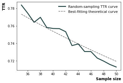
voc-D
Vocd score of lexical diversity derived from a series of TTR samplings and curve fittings
Step 1: Take 100 random samples of 35 words from the text. Compute the mean TTR from the 100 samples
Step 2: Repeat this procedure for samples of 36 words, 37 words, and so on, all the way to ntokens (recommended as 50 [default]). In each iteration, compute the TTR. Then get the mean TTR over the different number of tokens. So now we have an array of averaged TTR values for ntoken=35, ntoken=36,…, and so on until ntoken=50
Step 3: Find the best-fitting curve from the empirical function of TTR to word size (ntokens). The value of D that provides the best fit is the vocd score
Step 4: Repeat steps 1 to 3 for x number (default=3) of times before averaging D, which is the returned value
[20]:
lex.vocd(
    ntokens=50,  # Maximum number for the token/word size in the random samplings
    within_sample=100,  # Number of samples
    iterations=3,  # Number of times to repeat steps 1 to 3 before averaging
    seed=42  # Seed for reproducibility
)
[20]:
46.27679899103406
[21]:
lex.vocd()
[21]:
46.27679899103406
voc-D plot utility
Utility to plot empirical voc-D curve and the best fitting line
[22]:
lex.vocd_fig(
    ntokens=50,  # Maximum number for the token/word size in the random samplings
    within_sample=100,  # Number of samples
    seed=42,  # Seed for reproducibility
    savepath="images/vocd.png",
)
[22]:
<AxesSubplot:xlabel='Sample size', ylabel='TTR'>
HD-D
Hypergeometric distribution diversity (HD-D) score
(McCarthy and Jarvis 2007)
[23]:
lex.hdd(
    draws=42  # Number of random draws in the hypergeometric distribution
)
[23]:
0.7468703323966486
[ ]: